Input Optimization: Balancing Adversarial Discovery with Structured Sample Generation

What’s the best way to generate samples that meet structured criteria? In this post, the fine line between adversarial discovery and sample generation is demonstrated.

Motivating Example

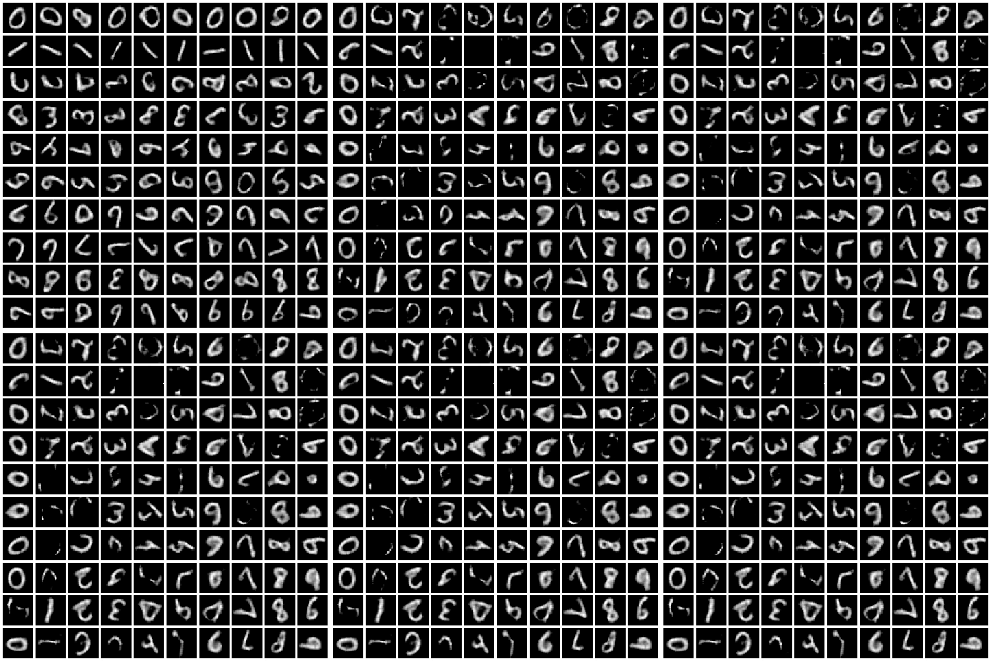
Above, we visualize a gradient-based optimization process attempting to interpolate between rotated MNIST digits. On the Y axis, we have initialized digits from 0 through 9, and on the X axis, we aim to generate a sample of class 0 through 9. It’s apparent that some digit targets are easier to transform to than others, like zeros: see how the outcome of mostly every optimization run in the first column looks like a 0 to a human. Notice too how the diagonal is minimally changed - this is optimal because our initial digit is already classified correctly. Additionally, notice how some examples end up with noncoherent shapes. What makes this optimization process work for some digits, while others become arbitrary blobs?

In this example, our gradient based optimization involves first pretraining an MNIST classifier $f_{\theta} : X \rightarrow Y$, where $X \in \mathbb{R}^{N \times N}, Y \in [0, 1, \dots, 9]$ on rotated MNIST shapes. We then initialize an optimization parameter $\hat{x} \in X$ to be a random digit from the dataset, and set a target $y \in Y$ represented as a one-hot vector. We fix the weights of our classifier $f_{\theta}$, then evaluate the cross-entropy loss between the predicted logits and our target one-hot vector:

This error is then backpropogated back to our input $\hat{x}$. Overall, recovering our “optimal” $x$ takes the form of something similar to maximum a-priori inference:

Here, I present why this problem can be broken into adversarial discovery and managing the data manifold. Note that we assume the manifold hypothesis.

Quick tangent: Why not just use Diffusion?

Denoising Diffusion models have been an increasingly popular way to sample from distributions and conditional distributions. They iteratively steer a randomly initialized $\hat{x}$ towards a sample from a distribution (without directly modeling distribution parameters like mean and variance, as is done in VAEs). However, what if you wanted to enforce that your samples meet some physical or symmetry constraints? Also, what if you want to better understand your data representation by seeing how it interpolates between classes (rather than just sampling $N$ points through a diffusion process)? This setup allows such things to be enforced during sample generation, as I will show later.

What’s the “optimal” x? (Adversarial discovery)

For the MNIST dataset, the decision boundaries between the features has been well studied. Current convolutional networks that have 2-3 layers and around 64 channels after downsampling can achieve close to 99% accuracy. Intuitively though, it’s a lot easier to add a few pixels here and there that will cause the model to misclassify our digit. The gradients from the optimization objective in Equation $\ref{eq:optobj}$ will actually steer our $\hat{x}$ towards the easiest solution that the classifier misclassifies, thus discovering an adversarial example. When this happens, it’s also called a Projected Gradient Descent (PGD) attack.

Therefore, we must find a way to measure if our sample is an adversarial example or not. This makes sense if we have some ground truth $f$ (say, from a simulated dataset) which we can evaluate $x$ on. As a reminder, $x$ is the outcome of our gradient descent on our surrogate function $f_\theta$ as Equation $\ref{eq:minobj}$ shows ¹. So, we will evaluate $x$ as follows to determine if it’s adversarial or not:

The takeaway is that this type of optimization works well when we’re simply using the surrogate as a differentiable form of a known ground-truth function. The problem is for inherent probabilistic functions (e.g. one digit class corresponds to multiple types of pictures), we don’t have this ground truth.

This is why metrics like Frenchet Inception Distance (FID) exist, which call the activations of an image classifier the “ground truth” $f_{FID} : \mathbb{R}^{N \times N} \rightarrow z$ where $z$ is the latent activation of the deepest layer of Inception v3. Embeddings aside for now, they compare the mean and variance of the generated data’s distribution (for a given $y$) against the actual distribution of the data of $y$ class. Therefore, they are measuring if the uncertainty of the modeled function matches the true uncertainty of the data (e.g. the distribution of the ground truth).

So, the type of optimization in Equation $\ref{eq:minobj}$ works best when the ground truth forward function $f$ is deterministic and the surrogate $f_\theta$ is also modeled deterministically. When $f$ is probabilistic, and we model $f_\theta$ deterministically, we are losing uncertainty estimation during backpropogation (e.g. taking the loss on the softmax of log probs instead of the log probs) ².

How do we propagate the uncertainty every iteration of gradient descent?

However, isn’t the softmax loss taken between two $\mathbb{R}^{10}$ vectors capture uncertainty? We want to award certainty. What if we add a term during backpropogation that penalizes uncertain estimations (e.g. where the difference between the min and max of the log probs is high)? But this already modeled because our target y is a one-hot vector (representing an absolute certainty for the class which we’re trying to achieve), so our loss is already penalizing uncertainty.

The real problem lies in that when we add a small noise, our model thinks it’s another class with high certainty. So how can we smooth that uncertainty estimation so that the uncertainty estimation has admissible and consistent properties? The answer is we train on data targets that aren’t represented as a one-hot vector, and instead, make the MNIST targets into probability distributions representing how close a human thinks that picture is to the digits in the class. So, a natural hypothesis would be that one-hot targets don’t give the model adequate information to interpolate in the space of uncertain estimations. Could this increase adversarial robustness without the need for explicit data augmentation?

There are a few works that tackle this through label-smoothing, which consists of reassigning a small portion of the max probability among other classes. This will result in better adversarial robustness, but a hypothesis is that it won’t be aligned with accurate probabilities. Therefore, this motivates the need for a human-labeled dataset of MNIST digits corresponding to vectors for how how likely it is that they’re another class.

How does this problem relate to the general accuracy vs robustness tradeoff?

It relates to our surrogate model $f_\theta$. We will consider the cases where our forward model is more accurate (generalizes better) vs more robust. If it’s more robust, then the gradients will steer more accurately steer the optimization away from adversarial examples. If it’s more accurate, then the gradients will more accurately steer the optimization towards the correct class of $y$. Ideally, we would like to have both.

Conclusions

In order to find the “optimal” x and not discover adversarial examples, $f_\theta$ must accurately model certainty (in the output representation layer) in an aligned manner. I recommend the creation of a dataset of feature MNIST images with target vectors representing a probability distribution over classes, where the targets are sourced from human labelers. This aligned signal will result in a more “human-optimal” x result from Equation $\ref{eq:minobj}$ (i.e. higher correlation with ground truth data).

Input representations (Managing the data manifold)

Gradient based optimization in a vector space relies, of course, on quality of the gradients produced through the forward model $f$. But what about the vector space itself? These aren’t completely disjoint things, since there does exist an interaction between the vector space and $\triangledown f$; if our gradients steer our generated sample into some subspace that is out of distribution (off the data manifold) for $f_\theta$ at timestep $t$, then $y_t$ will become some arbitrary, ill-defined value. This will be hard to rectify during the optimization progress $t+1 \dots T$.

Staying on-manifold

How does uncertainty estimation play into this? If we have accurate uncertainty estimates for out-of-distribution data, then as $\hat{x}$ gets closer to the distribution boundary, gradient descent should steer $\hat{x}$ away back towards the distribution. This would theoretically work because our loss target is a one-hot vector (which represents a target that’s very certain to be our target class). So, this motivates the need to train $f_\theta$ with out-of-distribution data whose target can be an arbitrarily “smooth” vector with almost equivalent probabilities for each class. This would enable high uncertainty estimations as $\hat{x}$ moves closer to the fringes of the data manifold.

Does this just simplify down to adversarial training? Not really. Adversarial training retains the same target signal for a perturbed input, with the goal of helping the network learn accurate mappings between off-manifold data and a known target ³. For example, we could add some small noise to an MNIST image of a 1 and set the target features as a one-hot vector representing 1 - or even better, as we talked about previously, a target vector whose argmax is 1 but has a more spread distribution over the other bins, which represents a higher uncertainty when noise is present ⁴.

Thickness of the manifold

We have shown progress in making our model give some meaningful representation for every point in the feature space, even if it’s off manifold, which will help gradient descent keep $\hat{x}$ on the data manifold. However, what if the data manifold is the same size as the feature space $X$? Then, it’s impossible to wander off during gradient descent.

However, we cannot change our data, so what if we reduce the size of our feature space instead? This is possible by representing our data in an embedding, where we lose the spatial structure of our MNIST data, but gain the ability to play with the feature space size (embedding size). Intuitively, we want the metric in our embedding space to be larger between digit images from different classes, and closer for images of the same class. A simple embedding for MNIST would be a 1-dimensional line with sequential bins for digit classes, where the embedding function $emb(\hat{x})$ could determine if an image belongs to a certain class, and give it a scalar value. $emb$ also necessarily needs to interpolate between digits in pixel space, so it can accurately reduce the dimensionality to a scalar between the appropriate digit bins. We don’t go too deep into MNIST embeddings, but read more here.

Instead, we focus on the size of the embedding. The more we reduce the dimensionality of our embedding (feature space), the less room gradient descent has to find a $\hat{x}$ that is outside the manifold $\mathcal{M}$ but inside the feature space $X$. In other words, we’re increasing the relative density of the manifold $\mathcal{M}$ within the feature space $X$, quantifed by the ratio

However, it’s important we don’t reduce it too much such that $D(\mathcal{M}, X) > 1$; otherwise, we will decrease representation performance by boxing in the data into a smaller space than it can naturally fit. There is an optimal latent size which can be found through hyperparameter tuning in the embedding function.

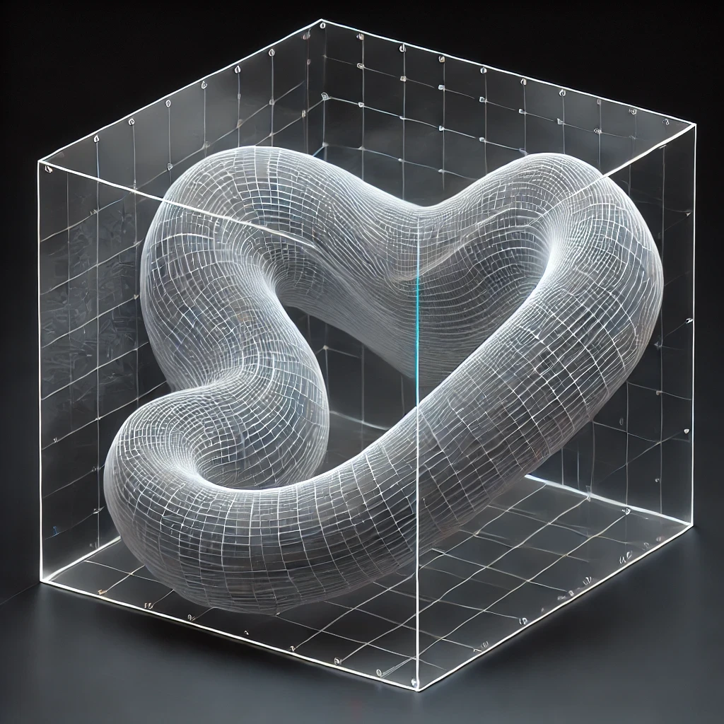
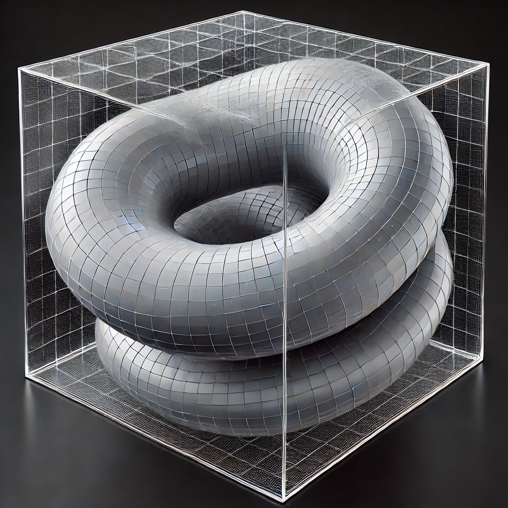
Below, we show a visualization of a feature space with lower density (left) versus higher density (right) where the grey manifold represents our data in the space. The manifold is not necessarily always smooth or connected, there may be disjoint pieces, or it might be more of a “tentacle” type of shape - these types of embeddings are difficult to study in higher dimensions.

The fine lines between out-of-distribution and off-manifold

When we’re doing adversarial robustness training on $f_\theta$, figuring out an embedding space for $\hat{x}$, and performing gradient descent, it’s important to accurately scope our problem so we can correct the necessary thing. We define the following:

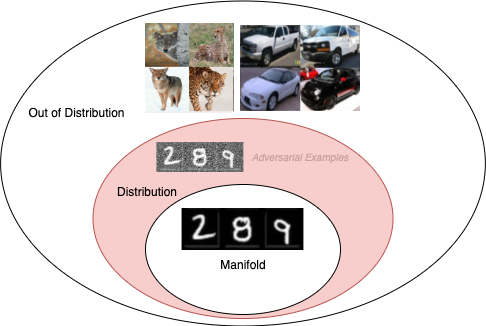
• Off-manifold: The space of data that can have the same semantic meaning as the training data, but is not produced by the natural signal that creates the data.
• Out-of-distribution: The space of data that has a different semantic meaning than the data which the model was trained on.
• Adversarial Example: A $\hat{x}$ that’s in-distribution but off the data manifold ⁵.

Here’s two examples to help differentiate:

• An attacker adds imperceivable noise to a few pixels of an MNIST image of a 3, and the model classifies it as a 9. This is an adversarial example (in-distribution, but off-manifold).
• A designer trains a model to classify MNIST. An attacker feeds in an image of a car, and the model classifies it as a two. The car image is an out-of-distribution sample (and thus, also off-manifold)

Conclusions

Train $f_\theta$ on out-of-distribution features, where the target represents a quantity of high uncertainty. Also, first embed your data into a lower dimensional space, then reduce the size of your embedding so the ratio in Equation $\ref{eq:ratio}$ is maximized. However, don’t reduce it too much such that the ratio becomes greater than 1.

Where does structure come into play?

Diffusion learns to sample from a distribution, and it is trained too using many samples from a distribution. But let us say we want to generate novel samples that meet a certain criteria / classification, say within some decision boundary of a downstream neural network $f_\theta$.

However, it will struggle to generate novel off-manifold samples unless it’s also trained on this data. This is a chicken and the egg problem. Instead, by using the gradients of $f_\theta$, we can iteratively move samples towards the desired boundary, all while meeting the structured criteria that’s enforced by $f_\theta$. This could manifest itself as an equivariant neural network.

($\dots$ in progress)